HyVR Computational methods¶

The first step in the HyVR algorithm is to load the model parameters, as defined in the *.ini initialisation file. These model parameters govern how the model will look like. A detailed documentation of all the options can be found here. Major strata contact surfaces are generated first. Architectural elements are then generated inside each stratum according to given probabilities. Finally, geometrical objects/hydrofacies assemblages like troughs, sheets, or channels are generated inside the architectural element.

After the model has been generated output values like facies, azimuth and dip are assigned to all grid points depending on which stratum/architectural element/object they belong to.

Based on these values (facies, azimuth, dip) and the settings in the [hydraulics] section, the hydralic parameters (porosity, isotropic hydraulic conductivity, full hydraulic conductivity tensor) are assigned, and potentially heterogeneity in these parameters on the given level.

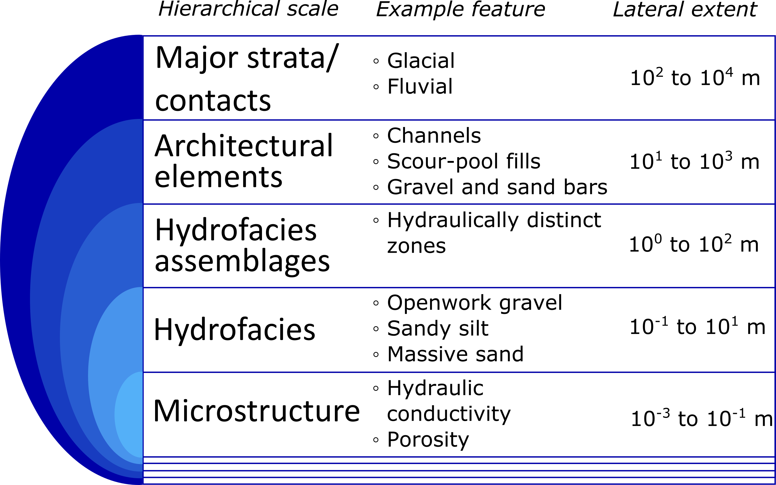
Hierarchical modeling framework implemented in HyVR.¶

Note that in this section model input parameters are denoted in the following manner: parameter-section.parameter.

Simulation of strata and architectural element contact surfaces¶

Strata are defined in the input parameter file by their bottom surface contact models and the architectural elements that are to be included within them. The top contact surface is then generated and all model cells between the upper and lower contact surface (which is the top of the next stratum) are assigned to the stratum.

Contact surfaces can either be flat or random. Multi-Gaussian random contact surfaces are generated using the spectral methods outlined by [DN93]. These methods require structural statistical parameters (i.e. mean and variance) for the quantity of interest, and a geostatistical covariance model. We used a Gaussian covariance model in the present study to produce smoothly varying surfaces:

\[R_{ss}(h)=\sigma^2_s \exp\left[ - \left[ \frac{\Delta x}{\lambda}\right]^2 \right]\]

where \(s\) is the random quantity of interest, \(\sigma^2_s\) is the variance of \(s\) (here elevation), \(\Delta x\) is the distance between the two points, and \(\lambda\) is the correlation length.

Once a bottom and top surface for a stratum is generated, architectural elements are created inside the stratum.

The architectural elements will be simulated based on input parameters defined for each stratum. This starts with the random choice of an architectural element from those defined; the probability of each architectural element being chosen is also defined in the input parameter file. The thickness of the architectural element is then drawn from a random normal distribution that is defined for each stratum in the input parameter file. To account for the erosive nature of many sedimentary environments the algorithm may erode the underlying units: here the ‘avulsion’ thickness \(th_{avulsion}\) is subtracted from the bottom and top of the architectural element \(z^{bot}_{AE}, z^{top}_{AE}\). Once the architectural element has been defined, contact surfaces are generated using the same procedure as used for strata contact surfaces. When the architectural element have been generated, the algorithm begins to simulate external hydrofacies assemblage geometries and hydrofacies.

Simulation of hydrofacies assemblages and hydrofacies geometries¶

The generation of hydrofacies assemblages and internal hydrofacies occurs stratum- and architectural-element-wise, beginning with the top-most architectural element in the top stratum. The simulation of individual hydrofacies assemblages is object-based, with random placement of features within the architectural element. Object-based methods have been implemented widely in subsurface simulation [JSD94][BHC17] as they are generally computationally efficient and relatively easy to parameterize. The HyVR program approximates hydrofacies assemblages with simple geometric shapes. Currently, three shapes are supported: troughs (truncated ellipsoids), channels (extruded parabolas), and sheets. Truncated ellipsoids and extruded parabolas are ‘erosive’ hydrofacies assemblages: this means that within the HyVR algorithm they are able to erode underlying units, and therefore the architectural element (and strata) boundaries may be altered during the course of the simulation.

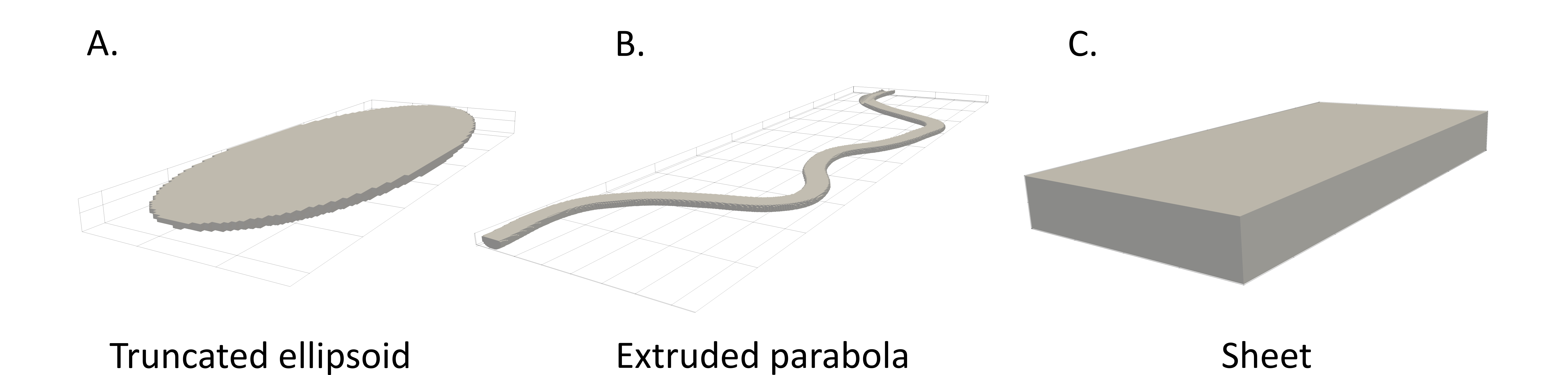
Geometries implemented in HyVR.¶

Four properties are assigned to each model grid cell during this simulation step: ae, ha_arr, hat_arr, facies, azimuth, and dip. The ae property denotes which architectural element (from strata.ae) has been assigned to a model grid cell. The ha_arr property is the unique identifier for each individual hydrofacies assemblage generated. hat_arr denotes the type of hydrofacies assemblage within the model grid cell is located. The facies property denotes which hydrofacies has been assigned to a model grid cell. The azimuth \(\kappa\) and dip \(\psi\) properties are associated with the bedding structure at each model grid cell and denote the angle of the bedding plane from the mean direction of flow and horizontal, respectively.

Truncated ellipsoids¶

Truncated ellipsoids are generated as a proxy for trough-like features. The method for generating the boundaries of these features has been described previously in [BHC17]. Generation starts at \(z^{bot}_{AE unit} +AE_{depth}\cdot\beta\) where \(AE_{depth}\) is the depth of the truncated ellipsoid geometry, and \(\beta\) is a buffer term that allows the user to control how much of the underlying unit is eroded. The centre of the truncated ellipsoid (\(x,y\) coordinates) and the paleoflow angle \(\alpha\) (i.e. major ellipsoid axis orientation) are drawn from a random uniform distribution and the boundary of the truncated ellipsoid is simulated. The internal structure of truncated ellipsoids can be defined in the following ways:

trough-wise homogeneous, with constant azimuth and dip;
bulb-dip, with azimuth and dip values based on the three-dimensional gradient at the ellipsoid boundary (‘bulb dip’);
bulb-sets, comprising nested alternating hydrofacies with \(\kappa\) and \(\psi\) values generated as for bulb-type;
dip-sets internal structure, where the features have a constant \(\kappa\) and \(\psi\) but the assigned hydrofacies alternate throughout the truncated ellipsoid.

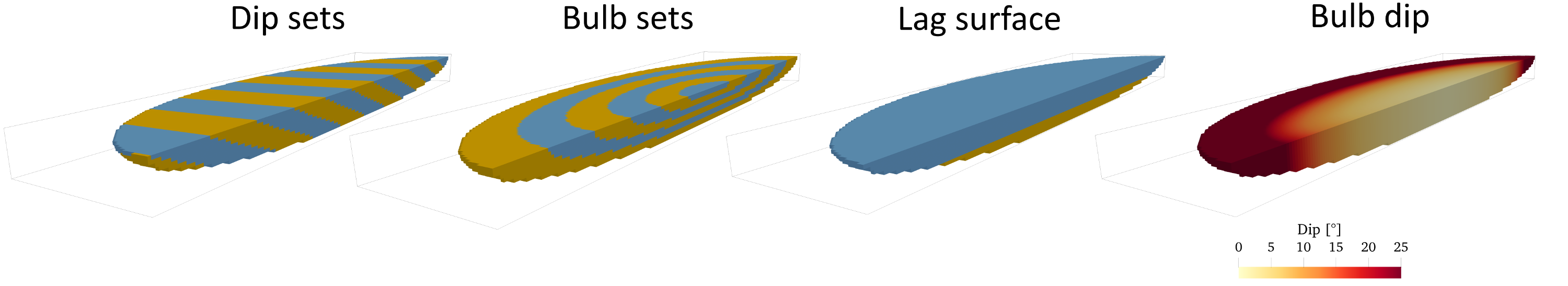
Internal structure of truncated ellipsoid hydrofacies assemblages.¶

Once a truncated ellipsoid has been generated, an aggradation thickness (trunc_ellip.agg) is added to the current simulation elevation \(z_{sim}\) and the next assemblage is simulated. This occurs until \(z_{sim} = z^{top}_{AE}\).

Truncated ellipsoid parameters

Bulb dip¶

Bulb hydrofacies assemblages is simulated by calculating the tangential vector at the boundary of the truncated ellipsoid and then the angle between the tangential vector and a horizontal plane. This angle is then compared with a ‘maximum dip angle’ (dip) and the smaller of these two values is assigned to all model grid cells within the hydrofacies assemblage with equivalent \(x,y\)-coordinates (i.e. column-wise). The tangential vector is calculated as gradient of

\[d^2(x,y,z) = \left(\frac{x}{a}\right)^2 + \left(\frac{y}{b}\right)^2 + \left(\frac{z}{c}\right)^2\]

Bulb sets¶

Nested-bulb-like layers are simulated by subdividing the depth of the truncated ellipsoid into a series with a set thickness trunc_ellip.bulbset_d. Truncated ellipsoids are simulated consecutively with the same center point and paleoflow \(\alpha\) value, starting with the deepest assemblage. With each simulation, a scaling factor is calculated by dividing the new depth with the total depth of the assemblage. This scaling factor is applied to the length and width parameters of the truncated ellipsoid. Each newly generated ellipsoid subsumes the previous. Each nested assemblage represents a constant hydrofacies, however the orientation of these hydrofacies may differ within the entire hydrofacies assemblage, to create bulb-like features that have been reported in the field. The dip of the nested ellipsoids defaults to that determined by the three-dimension gradient at the nested-ellipsoid boundary.

Dip sets¶

Refer to dipset section.

Extruded parabolas¶

Parabolas extruded along arbitrary curves with variable sinuosity are useful to represent channels. Extruded parabola centrelines in HyVR are parameterized using the disturbed periodic model implemented by [Fer76]:

\[\theta + \frac{2h}{k} \frac{d\theta}{ds} + \frac{1}{k^2} \frac{d^2\theta}{ds^2} = \epsilon(s)\]

with curve direction \(\theta\), damping factor \(h \in [0,1]\), \(k = 2\pi/\lambda\) is the wavenumber with \(\lambda\) the frequency of the undamped sine wave, and \(s\) is the distance along the curve. This model can be approximated using the following second-order autoregressive model described in Equation 15 of [Fer76]:

\[\theta_i - b_1 \theta_{i-1} - b_2\theta{i-2} = \epsilon_i\]

with:

\[b_1 = 2 e^{-kh}\cos(k\arcsin(h))\]

\[b_2 = -e^{-2kh}\]

This method was also used by [PBD09] for the simulation of alluvial depositional features. Model grid cells are assigned to the extruded parabola if the following conditions are met:

\[D^2 \leq \frac{w_{ch}^2}{4} + \frac{w_{ch}^2 (z_{cell} - z_{ch})}{4 d_{ch}}\quad\text{and }\quad z_{cell} \leq z_{ch}\]

where \(D^2\) is the two-dimensional (\(x,y\)) distance from the cell to the extruded parabola centerline, \(w_{ch}\) and \(d_{ch}\) are the extruded parabola width and depth respectively, \(z_{ch}\) and \(z_{cell}\) are the elevations of the extruded parabola top and node respectively. Two-dimensional ‘channel velocities’ \(\vec{v}\) are evaluated at the centerline and then interpolated to grid cells using an inverse-distance-weighted interpolation. Azimuth values are calculated by taking the arctangent of the two-dimensional channel velocity at a given point. Dip values of grid cells within the extruded parabola are assigned based on input parameters. If alternating hydrofacies are to be simulated they are constructed by creating planes that are evenly spaced along the extruded parabola centerline.

The HyVR algorithm generates extruded parabolas starting from \(z^{bot}_{AE unit} +AE_{depth}\cdot\beta\), as for truncated ellipsoids. However, to account for the multiple extruded parabolas that are often concurrently present in many river systems, multiple extruded parabolas can be generated at each simulation depth (ext_par.channel_no). The starting \(x,y\) coordinates for the centerlines are drawn from a random uniform distribution such that \(x\in[-50,0]\) and \(y\in[0,Y]\). Extruded parabola geometries are then assigned sequentially to the model grid cells; note that in HyVR there is no interaction of extruded parabolas, and subsequent extruded parabolas will supersede (or ‘erode’) those previously generated. Once the predefined number of extruded parabolas stipulated by ext_par.channel_no has been simulated a three-dimensional migration vector ext_par.mig is added to the extruded parabola centerlines and the extruded parabola assignment to model grid cells begins again. The reuse of the extruded parabola centerline trajectories is more efficient than re-simulating these values at each \(z_{sim}\). This continues until \(z_{sim} = z^{top}_{seq}\).

Extruded parabola parameters

Sheets¶

Sheets are comparatively simple to generate as they are laterally continuous across the entire model domain (depending on strata boundaries). The internal structure of sheet features may be massive (i.e. without internal structure), or laminations can be generated. In the HyVR algorithm laminations are simulated sequentially by assigning all model grid cells between a specific elevation interval the appropriate hydrofacies codes. Dipping set structures can also be incorporated into these features. Sheets may differ in internal orientation, as specified in the input parameters.

Sheet parameters

Internal structure¶

The internal structure of the hydrofacies assemblages is distinguished by hydrofacies. The internal structure of an hydrofacies assemblage may be homogeneous, dipping or ellipsoidal (for truncated ellipsoid only). Additionally, lag surfaces composed of different hydrofacies may be simulated in erosive (i.e. extruded parabola, truncated ellipsoid) hydrofacies assemblage.

Dipset¶

Architectural elements may be populated with dipping hydrofacies structures. Such structures are generated by creating planes at regular intervals throughout the architectural element, as defined by element.dipset_d. In truncated ellipsoids the planes are constructed along the centerline of the element, perpendicular to the paleoflow angle \(\alpha\). In extruded parabola elements, the planes are constructed along the centerline and are perpendicular to \(\vec{v}(x)\). The distance from the centre of each model grid cell to all planes is calculated and then the model grid cells between planes are assigned a hydrofacies value.

Lag surfaces¶

Lag surfaces can be set for erosive hydrofacies assemblages by setting the element.lag parameter. This parameter consists of two values:

The thickness of the lag surface from the element base; and
The hydrofacies identifier to be assigned.

Lag surfaces cannot have any internal dipping structure.

Alternating hydrofacies¶

Sedimentary deposits can often exhibit cyclicity in their features; therefore, HyVR allows alternating hydrofacies to be simulated. This is controlled by sequentially assigning hydrofacies within each hydrofacies assemblage, starting with a hydrofacies randomly selected from those to be simulated in the architectural element (element.facies). The hydrofacies which is assigned next is drawn from a subset of hydrofacies specified in the element.altfacies input parameter. For each hydrofacies in element.facies, a list of alternating hydrofacies (i.e., which hydrofacies can follow the present one) is stipulated. By only specifying one hydrofacies ID in the element.altfacies, it guarantees that that ID will be selected. The figure below gives three examples of different input parameters.

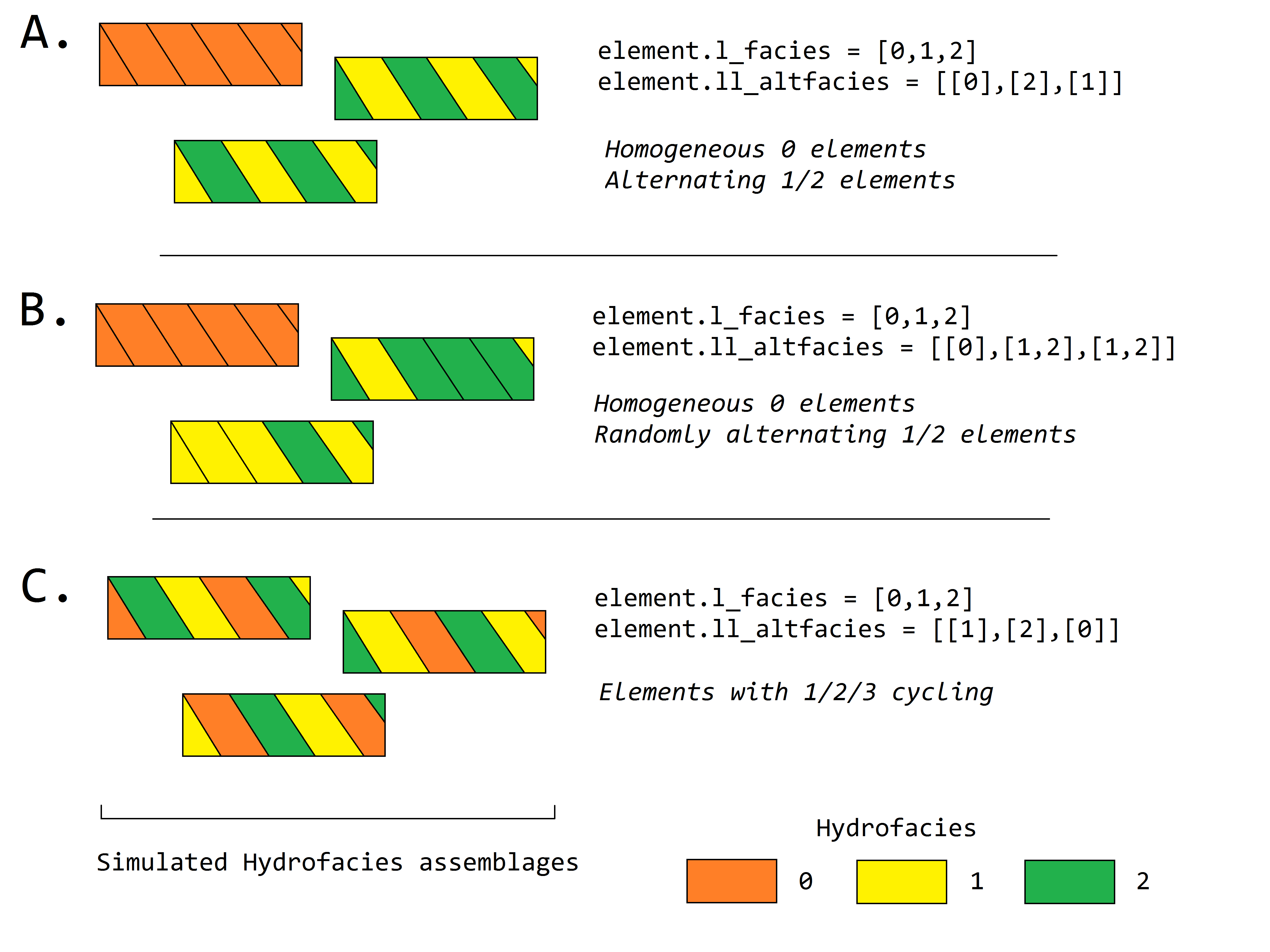
Variations on alternating hydrofacies in architectural elements¶

Linear trends¶

The HyVR algorithm allows for linear trends in geometry sizes with increasing elevation by setting the element.geo_ztrend parameter. This parameter comprises a bottom and top factor \(\xi_{bottom},\xi_{top}\) that multiply the usual geometry dimensions. For intermediate elevations the \(z\) factor is calculated through a linear interpolation of \(\xi_{bottom},\xi_{top}\). The parameters of each geometry may be set for each individual architectural element included in the model parameter file.

Simulation of hydraulic parameters¶

Hydraulic parameters are simulated once all features have been generated. The distributed hydraulic parameter outputs of HyVR are: the isotropic hydraulic conductivity \(K_{iso}(x,y,z)\); porosity \(\theta(x,y,z)\); and the full hydraulic conductivity tensor \(\textbf{K}(x,y,z)\), defined for each model grid cell.

Microstructure of hydraulic parameters is first simulated for each individual hydrofacies assemblage (as present in the mat storage array) simulated in the previous steps. Spatially varying \(\ln(K_{iso})\) and \(\theta\) fields are generated for each hydrofacies present in an hydrofacies assemblage using spectral methods to simulate random multi-Gaussian fields with an exponential covariance model:

\[R_{ss}(h)=\sigma^2_s \exp\left[ - \left| \frac{\Delta x}{\lambda}\right| \right]\]

An anisotropic ratio is also assigned to each model grid cell according to the hydrofacies present; these ratios are globally constant for each hydrofacies.

Microstructure may also be assigned to model grid cells that are not within hydrofacies assemblage. This background heterogeneity is simulated for each architectural element using values defined for each architectural element type (element.bg). Simulation methods are the same as for within-assemblage heterogeneity.

Spatial trends may also be applied once isotropic hydraulic-conductivity values have been assigned to all model grid cells. As for trends in hydrofacies assemblage geometry, trends are assigned using a linearly-interpolated factor \(\xi_{start},\xi_{end}\) in the \(x\)- and/or \(z\)-directions. The value of each model grid cell is then multiplied by the trend factors.

Hydraulic-conductivity tensors¶

Full hydraulic-conductivity tensors for each model grid cell are calculated by multiplying the isotropic hydraulic conductivity \(K^{iso}\), with a rotated anisotropy matrix \(\textbf{M}\):

\[\textbf{K}_i =K^{iso}_i\textbf{R}_i\textbf{M}_i\textbf{R}_i^T\]

\[\begin{split}\textbf{R}_i = \begin{bmatrix} \cos(\kappa_i)\cos(\psi_i) & \sin(\kappa_i) & \cos(\kappa_i)\sin(\psi_i)\\ -\sin(\kappa_i)\cos(\psi_i) & \cos(\kappa_i) & -\sin(\kappa_i)\sin(\psi_i)\\ -\sin(\psi_i) & 0 & \cos(\psi_i) \end{bmatrix}\end{split}\]

Parameters \(\psi_i\) and \(\kappa_i\) are the simulated bedding structures (dip and azimuth, respectively). The anisotropy matrix \(\textbf{M}_i\) is diagonal with lateral terms set as equivalent (i.e. \(K_{xx} = K_{yy}\)). This approach is identical to that of [BHC17]. Once this has been completed, the simulated parameter files are saved and can be used for groundwater flow and solute transport simulations.